Multi-Mode Interference
Introduction
Multi-mode interferometer, due to their advantages of low insertion loss, wide bandwidth, simple fabrication process, and good tolerance, have been widely used in important optical devices such as optical switches and wavelength-division multiplexers.
The main performance parameters of multi-mode interference couplers include insertion Loss, imbalance, device dimensions, operating bandwidth.
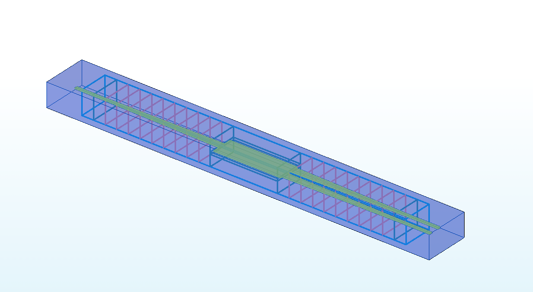 |  |
|---|
Simulation Methods
With the EME module, the corresponding cell groups and cell numbers can be set up with the structure, and a parameter sweep can be performed in the propagation sweep to obtain the S-parameters of the device. This parameter sweep helps optimize the core dimensions of the multi-mode interferometer, ensuring desired performance characteristics.
Alternatively, FDTD module can be conducted to obtain the intensity distribution of the optical field and the transmittance at each port. This allows the verification of the optimized results for the multi-mode interferometer.
After data processing, performance parameters such as the imbalance, insertion loss, and bandwidth of the device can be determined.
Multi-Mode Interference(EME module)
The simulation design of a multimode interference coupler typically employs the EME module. This allows for a rapid scan of the length of the multimode interference region to quickly identify the optimal length for beam splitting. Therefore, in the following code, we will learn how to create a Multi-Mode Interference (MMI) simulation and output the results for data processing.
1. Basic Operations
1.1 Import File
Once you have installed and configured the environment, import the python code and the GDS layout. The example library and related model code are usually located in the directory :examples/func_demo. The GDS file is generally imported into the path :examples/examples_gds
1.2 SDK Initialization
Create a new terminal and run the code after you import the python script and GDS file. Max-Optics SDK may take some time to connect the service.
2.Code Description
Now let's learn the meaning of functions and parameters that correspond to the code.
2.1 import Modules
To begin, we need to use the import command to call the relevant functional modules. For instance, we import the typing , os and time module in python. At the same time ,we import the customized module maxoptics_sdk.all and maxoptics_sdk.helper.
import maxoptics_sdk.all as mo
from maxoptics_sdk.helper import timed, with_path
import os
import time
from typing import NamedTuple
The maxoptics_sdk package provides all in one optical simulation with Python.
The os module provides a way to use operating system-dependent functionality such as reading or writing to the file system, working with environment variables, and executing system commands.
The time module provides various functions to work with time-related operations and to measure time intervals.
The typing module provides support for type hints and annotations, which are used to indicate the expected types of variables, function arguments, and return values in your code.
2.2 Define Simulation
Firstly, We define parameters and give them a default value, such as the simulation wavelength and number of modes. Note that we can override this value in the following code.
@timed
@with_path
def simulation(*,wavelength=1.55,wavelength_span=0.1,number_of_modes=10,global_mesh_grid=0.155,local_mesh_grid=0.01,run_options: "RunOptions",**kwargs):
The provided code contains comments that define the simulation parameters. Let's explain each of these parameters.
The function simulation is used to define the simulation parameters for the program.
The run_mode parameter determines the type of calculation resources to be used.
The wavelength parameter specifies the wavelength of the input light in micrometers.
The number_of_trial_modes parameter sets the number of modes to be calculated.
The **kwargs is a special syntax used in function definitions to accept an arbitrary number of keyword arguments as a dictionary.
2.3 Define Parameters
Define commonly used parameters in this region, such as the mesh grid of the simulation boundary, the start time of the simulation, the path and name for the simulation output, the path to the imported GDS layout, and other parameters required for structural parameterized modeling.
If you need to calculate the bandwith of the device in the EME simulation, you can also decide the wavelength for sweeping in this section.
# region --- General Parameters ---
path = kwargs["path"]
simu_name = "EME_1X2MMI"
time_str = time.strftime("%Y%m%d_%H%M%S", time.localtime())
project_name = f'{simu_name}_{time_str}'
plot_path = f'{path}/plots/{project_name}/'
gds_file_root_path = os.path.abspath(os.path.join(path, '..'))
gds_file = gds_file_root_path + "/examples_gds/1X2MMI.gds"
kL = [f"0{k}" for k in range(5)]
# endregion
The code defines several parameters and variables necessary for the simulation process. The global_mesh_grid parameter represents the mesh in the EME simulation region. Similarly, the local_mesh_grid parameter denotes the customized mesh for user defined region.
The path variable defines the file path for the simulation, while simu_name specifies the name of the simulation file.
The time_str variable is used to obtain the current time as a timestamp for the simulation.
The project_name variable assigns a name to the project for the simulation output.
The plot_path variable determines the directory where the simulation result plots will be saved.
The gds_file_root_path variable defines the path for importing the GDS layout.
The parameters wavelength_start,wavelength_stop,wavelength_points are for sweeping.
These parameters and variables together facilitate the successful execution and organization of the simulation process.
2.4 Creat Project
You can create a new project using the Project function of Max's software development toolkit.
# region --- Project ---
pj = mo.Project(name=project_name)
# endregion
2.5 Define Materials
Let's proceed to the next step, where we set up the materials required for the simulation. In this case, we will directly use relevant materials from the MO material library.
# region --- Material ---
mt = pj.Material()
mt.add_nondispersion(name="Si", data=[(3.454996, 0)], order=2)
mt.add_nondispersion(name="SiO2", data=[(1.444991, 0)], order=2)
mt.add_lib(name="Air", data=mo.Material.Air, order=2)
# endregion
The add_lib contains three parameters name,data and order.
The data calls up the property of simulation materials in the MO material library.
The Order parameter determines the mesh order for the material during the simulation.
As the same, we also support users to customize the material with add_nondispersionfunction.
2.6 Create Model
Next, we will create the MMI model.
# region --- Structure ---
st = pj.Structure()
st.add_geometry(name="box", type="gds_file",
                property={"general": {"path": gds_file, "cell_name": "TOP", "layer_name": (1, 1)},
                            "geometry": {"x": 0, "y": 0, "z": 0, "z_span": 4},
                            "material": {"material": mt["SiO2"], "mesh_order": 2}})
st.add_geometry(name="psr", type="gds_file",
                property={"general": {"path": gds_file, "cell_name": "TOP", "layer_name": (2, 1)},
                            "geometry": {"x": 0, "y": 0, "z": 0.11, "z_span": 0.22},
                            "material": {"material": mt["Si"], "mesh_order": 2}})
# endregion
We can import the MMI layout from the GDS file.
The name parameter defines the structure name.
The type parameter specifies the structure type.
The path, cell_name, and layer_name parameters point to the GDS file and specify the relevant layers and cell names used in the layout.
The geometry parameter sets the structure's coordinates.
The material parameter specifies the material properties
The mesh_order parameter sets the mesh order for the simulation.
2.7 Simulation
# region --- Simulation ---
simu = pj.Simulation()
simu.add(name=simu_name,type="EME",
        property={"background_material": mt["Air"],
                    "mesh_settings": {"mesh_factor": 1.2,"mesh_refinement": {"mesh_refinement": "curve_mesh",},},
        "geometry": {"x_min": 3, "y": 0, "y_span": 5, "z": 0, "z_span": 4},
        "boundary_conditions": {"y_min_bc": "PML", "y_max_bc": "PML", "z_min_bc": "PML", "z_max_bc": "PML",
                                            "pml_settings": {"pml_kappa": 2, "pml_sigma": 5, "pml_layer": 12, "pml_polynomial": 3}},
        "general": {"wavelength": wavelength,"wavelength_offset": 0.0003,"use_wavelength_sweep": True,},
        "eme_setup": {"cell_geometry": {
                        "cell_group_definition": [
                            {"span": 2, "cell_number": 1, "number_of_modes": number_of_modes, "sc": "none"},
                            {"span": 20, "cell_number": 10, "number_of_modes": number_of_modes, "sc": "sub_cell"},
                            {"span": 11.5, "cell_number": 1, "number_of_modes": number_of_modes, "sc": "none"},
                            {"span": 20, "cell_number": 10, "number_of_modes": number_of_modes, "sc": "sub_cell"},
                            {"span": 2, "cell_number": 1, "number_of_modes": number_of_modes, "sc": "none"},]}},
        "transverse_mesh_setting": {"global_mesh_uniform_grid": {"dy": global_mesh_grid, "dz": 0.05}},},)
# endregion
The name parameter defines the name of the simulation module.
The property parameter specifies the general property of the simulation module, such as the geometry of cell, wavelength and so on.
The cell_group_definition parameter specifies the general property of the cell group.
The number_of_modes parameter specifies the general property of the simulation module within the structure, such as the geometry of cell, wavelength and so on.
The sc parameter sets the subcell method in EME simulation. Selections are ['none', 'sub_cell'].
2.8 Add Sub-mesh
# region --- Sub Mesh ---
lm = pj.LocalMesh()
lm.add(name="sub_mesh",
        property={"general": {"dx": local_mesh_grid,"dy": local_mesh_grid, "dz": local_mesh_grid},
                    "geometry": {"x": 30.75, "x_span": 11.5, "y": 0, "y_span": 5, "z": 0.11, "z_span": 0.4},},)
# endregion
In this code segment, we add a sub-mesh.
The name parameter defines the name of the mesh.
The general parameter specifies the grid accuracy in the xyz directions .
The geometry parameter sets the coordinates of the sub-mesh.
2.9 EME Port
Then, we add the EME Port for calculating modes in the simulation.
# region --- Port ---
pjp = pj.Port()
pjp.add(name="input_port", type="eme_port",
        property={"modal_analysis": {"wavelength": wavelength,},
                    "geometry": {"port_location": "left", "use_full_simulation_span": True,},
                    "eme_port": {"general": {"mode_selection": "fundamental_TE", "number_of_trial_modes": number_of_modes},
                                "advanced": {"offset": 0.1,}}})
pjp.add(name="output_port1", type="eme_port",
        property={"modal_analysis": {"wavelength": wavelength,},
                    "geometry": {"port_location": "right", "use_full_simulation_span": False, "y": 0.9, "y_span": 2, "z": 0.11, "z_span": 2 },
                    "eme_port": {"general": {"mode_selection": "fundamental_TE", "number_of_trial_modes": number_of_modes},
                    "advanced": {"offset": 0,}}})
pjp.add(name="output_port2", type="eme_port",
        property={"modal_analysis": { "wavelength": wavelength, },
                    "geometry": {"port_location": "right", "use_full_simulation_span": False,"y": -0.9, "y_span": 2, "z": 0.11, "z_span": 2},
                    "eme_port": {"general": {"mode_selection": "fundamental_TE", "number_of_trial_modes": number_of_modes},
                        "advanced": {"offset": 0, }}})
# endregion
The name parameter defines the name of the EME port.
The port_location parameter sets the location type of EME port. Selections are ['left', 'right'].
The use_full_simulation_span parameter confirms whether to use full simulation span.
The mode_selection parameter decides the mode which propagates in the waveguide. Selections are ['fundamental', 'fundamental_TE', 'fundamental_TM', 'fundamental_TE_and_TM', 'user_select', 'user_import'].
The number_of_trial_modes parameter determines the calculated number of modes around the refractive index.
2.10 Add Monitor
In this region, we add the profile monitors for the EME simulation.
# region --- Monitor ---
mn = pj.Monitor()
mn.add(name="z_normal", type="profile_monitor",
        property={"geometry": {"monitor_type": "2d_z_normal",
                                "x_resolution": 100,"x": 30.75, "x_span": 55.5, "y": 0, "y_span": 5, "z": 0.11, "z_span":0 }})
for i, pos in enumerate([10, 17.5, 23.5, 34.5, 39.5]):
    mn.add(name="section"+str(i+1), type="profile_monitor",
            property={"geometry": {"monitor_type": "2d_x_normal", "x_resolution": 100,
                                    "x": pos, "x_span": 0, "y": 0, "y_span": 5, "z": 0.11, "z_span": 2}})
# endregion
The monitor_type parameter selects the profile monitor type and the orientation.Selections are ['2d_x_normal', '2d_y_normal', '2d_z_normal', 'x', 'y', 'z'].
The x_resolution parameter decides the resolution of output simulation results in profile monitor.
2.11 EME Analysis
Next, we run the analysis for this simulation.In this part, we can set detailed information of wavelength sweep,groupspan sweep,periodicity and so on.
# region --- EME Analys ---
grating_periods = 1
eme_base_res = simu[simu_name].run()
analysis = pj.Analysis()
analysis.add(name="eme_propagate", type="eme_analysis",
                property={"workflow_id": eme_base_res.workflow_id, "eme_propagate": run_options.run,
                        "periodicity": {"periodicity": True,
                                        "periodic_group_definition": [{"start_cell_group": "group_span_1", "end_cell_group": "group_span_1", "periods": grating_periods}]},
                        "group_span_sweep": {"group_span_sweep": run_options.run_length_sweep,
                                            "parameter": "group_span_3", "start": 10, "stop": 100, "number_of_points": 101},
                        "wavelength_sweep": {"wavelength_sweep": run_options.run_wavelength_sweep,
                                            "start": wavelength-wavelength_span/2, "stop": wavelength+wavelength_span/2, "number_of_wavelength_points": 11},})
# endregion
2.12 Calculate Mode
In this region, we calculate the modes of ports. Before running EME simulation calculations, we can calculate the mode field distribution of the port by setting the type of mode selection to True and other simulations to False.
# region --- Calculate Mode ---
if run_options.calculate_modes:
    for port in ["input_port", "output_port1","output_port2"]:
        k = kL[2]
        simu[simu_name].preview_modes(port_name=port, data="calculate_modes",
                                        savepath=f"{plot_path}{k}_modeprofile_fdeonly_{port}",
                                        attribute="E", mode=0,)
        simu[simu_name].preview_modes(port_name=port, data="calculate_modes",
                                        savepath=f"{plot_path}{k}_Preview_{port}_neff",
                                        show=False, export_csv=True,)
# endregion
2.13 Extract Results
This region is uesd to retrieve and store the simulation results.
# region --- See Results --
eme_res = analysis["eme_propagate"].run()
if run_options.extract:
    if run_options.run:
        eme_res.extract(data="eme_propagate:cell_power_total",
                        savepath=f"{plot_path}00_cell_power_total",
                        target="line", toward="forward", export_csv=True,)
        eme_res.extract(data="eme_propagate:cell_power_mode",
                        savepath=f"{plot_path}01_cell_power_mode",
                        target="intensity", toward="forward", export_csv=True,)
        eme_res.extract(data="eme_propagate:cell_neff",
                        savepath=f"{plot_path}02_cell_neff", target="intensity", export_csv=True,)

        for port_name in ["input_port",  "output_port1","output_port2"]:
            res = eme_res.extract(data="eme_propagate:port_mesh_structure",
                                    savepath=f"{plot_path}03_eme_structure_{port_name}",
                                    port_name=port_name, target="intensity",)

        eme_res.extract(data="eme_propagate:smatrix",
                        savepath=plot_path + "04_eme_smatrix_intensity", target="intensity", export_csv=True)
        eme_res.extract(data="eme_propagate:monitor",
                        savepath=plot_path + "05_eme_z_normal",
                        monitor_name="z_normal", attribute="E", export_csv=True)

        for i in range(5):
            eme_res.extract(data="eme_propagate:monitor",
                            savepath=plot_path + "06_eme_section"+str(i+1),
                            monitor_name="section"+str(i+1), attribute="E", export_csv=True)

    if run_options.run_wavelength_sweep:
        eme_res.extract(data="wavelength_sweep:sweep",
                        savepath=plot_path + "07_wavelength_sweep", plot_x="wavelength", export_csv=True,)
    if run_options.run_length_sweep:
        eme_res.extract(data="propagation_sweep:sweep",
                        savepath=plot_path + "08_length_sweep", plot_x="length", export_csv=True,)
# endregion
return project_name
The extract function allows you to extract specific simulation results and store them for further analysis.
The data parameter is to decide what type/field data will be extracted.
The savepath parameter specifies the save path of picture.
The monitor_name parameter specifies the name of monitor which provides the data needed.
The plot_x parameter specifies the data of x axis.
The export_csv parameter is to decide whether to export a csv. Default as False.
2.14 Switches
In this section of the code, the simulation function is called and executed, which allows you to reset relevant parameters for more convenient parameter scanning and optimization design. We also support control switches for various functionalities at the end of the code, and you can use configuration flags(True or False). These flags can be used to turn specific functionalities on or off, making it easier to check the model and perform efficient calculations.
class RunOptions(NamedTuple):
    calculate_modes: bool
    run: bool
    run_length_sweep: bool
    run_wavelength_sweep: bool
    extract: bool


if __name__ == "__main__":
    simulation(run_mode="local", wavelength=1.55, wavelength_span=0.1,
               global_mesh_grid=0.1, local_mesh_grid=0.02, number_of_modes=10,
               run_options=RunOptions(calculate_modes=True, run=True, run_length_sweep=True, run_wavelength_sweep=True, extract=True,),)
By turning on/off the relevant functionalities, you can control the simulation process and obtain the desired results. For example, the calculate_modes determines whether to calculate the modes. The run determines whether to do the EME propagation in the program. run_wavelength_sweep is used to enable wavelength scanning, and extract is used to control data extraction. Properly utilizing these switches can help you inspect the simulation effectively.
3.Output Results
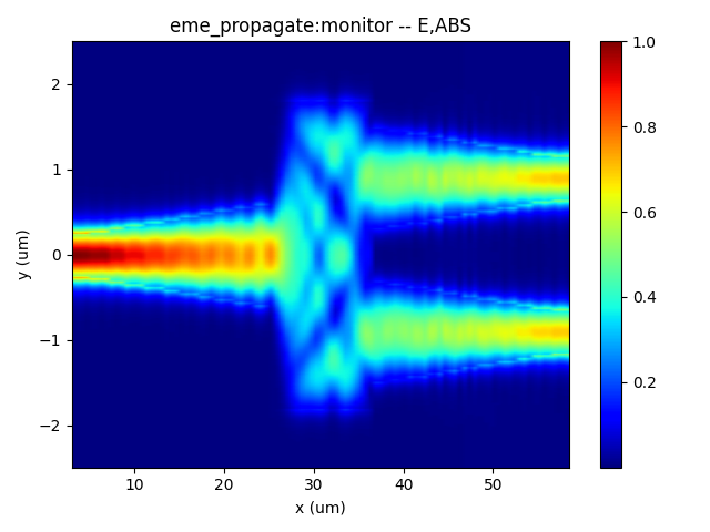
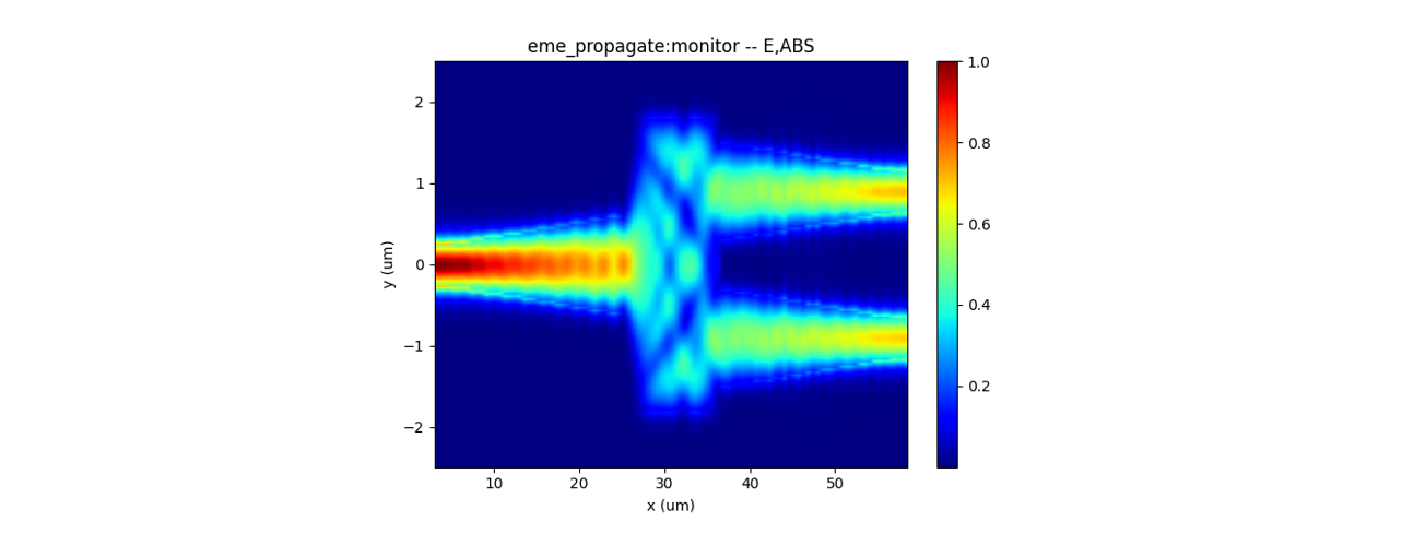
- the z-normal E intensity of EME propagation
 |
|---|
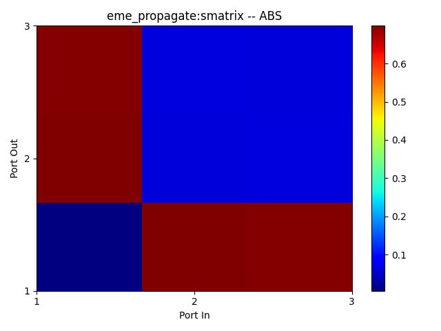
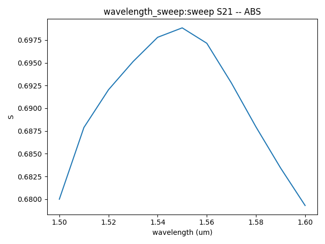
- The S matrix of EME propagation and the S parameters and transmission at different wavelength..
As shown in the figure below, the S-matrix is a 3∙3 matrix.
 |  |
|---|
The S21 parameter represents the absolute value of the transmission coefficient from port 1 input to port 2 output. Due to the symmetry of the structure, S31=S21. The transmission result is shown in the left picture below which is calculted form the S parameter about the one of output ports. Therefore, we can obtain the insert loss is about 0.114 dB at 1.55 micrometer wavelength.
Supplement
To view a function's definition and supported parameters or a parameter dictionary, you can right-click on its name and select "Go to Definition" or press "Ctrl" while left-clicking on its name to view its definition, showing the available parameters and their descriptions.